Issue 4, June 1984 - Plotting in 3D (part 2 of 2)
| Home | Contents | KwikPik |
| Issue 3 | part 1: "Graphics & Mathematics" |
| This program is available on "ZIPi'T'ape", which holds the files for both parts of the article. | |
|
In Part One (published in last month's
Your Spectrum), the perspective was
demonstrated using the 'plane plotting'
routine. This time, the spherical co-ordinates are chosen to generate a
variety of symmetrical 3D objects and
also to provide relatively simple transformations (scaling, rotation and
translation). The routines are used in the
main part of the program (listed in Part
One) and the co-ordinates system is
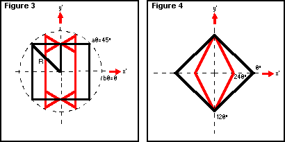
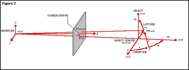
depicted in Figure 2. Object generation starts at line 90 with the set of INPUT statements defining object parameters chosen by the observer. The parameters asked for in the program will produce data for the generation of: - the number of vertical sections, sb - the number of sides in each section, sa - the starting longitude; that is, the longitude bf the first vertical section, b0 - the starting latitude; that is, the latitude of the origin of the DRAW vector representing the first side of the polygon, a0. This can be seen in Figure 3. sb = 3 sa = 4 b0 = 0 a0 = 45° Figure 3 will generate three vertical sections - at 0°, 120° and 240° - each section being represented by a wire- frame figure of a square orientated so that it has two horizontal and two vertical sides. If you were to make a0 equal to 0°, you would produce squares with sides at 45° to the horizontal (see Figure 4). The object size will obviously be determined by R (line 100) and the apparent size using perspective will also depend on the object distance from |

Continuing on his quest to make perspective a reality on the Spectrum, Damir Skrgatic tackles the subject of symmetrical figures generated through the application of spherical co-ordinates. |
|
|---|---|---|
|
the observer, z0 (line 90). Varying the
value of z0 is equivalent to 'zooming'
with a camera - translation along
depth. The x and y translation is achieved
by varying x0 and y0 respectively (the
centre of the screen is x0=0 and y0=0). So now, with reference to the 3D Plotting program published in the first part of this article (see last issue), here follows a detailed breakdown of the |
lines which deal specifically with
spherical co-ordinates. Lines 170 and 180 convert chosen numbers, sb and sa, into angular increments in degrees, db and da, used by the FOR-NEXT loops in lines 190 and 200. Lines 210 to 270 convert spherical co-ordinates R, a and b into rectangular co-ordinates x, y and z (and their increments: dx, dy and dz), so that the object |
|
|
||
|
||

can be plotted in perspective in a similar manner to the plane drawing routines demonstrated in Part One. Lines 220 to 240 are standard equations converting spherical co-ordinates into rectangular co-ordinates and can be derived from Figure 2 using trigonometry. (Note that all angles under SIN and COS have been converted to radians = PI/180 * angle in degrees.) Lines 250 to 270 compute cartesian increments (vectors) dx, dy and dz, corresponding to the latitude increment, da. (This is a good example of a very cumbersome number crunching exercise which a home computer can do easily, although not as fast as CAD dedicated machines.) Note that all results are still in millimetres. Lines 280 to 360 provide clipping outside the viewing pyramid and the |
FURTHER PARAMETER EXAMPLES FOR THE 3D PLOTTING PROGRAM*
|
|||||||||||||
|---|---|---|---|---|---|---|---|---|---|---|---|---|---|---|
|
limits used correspond to d = 500mm
and the Spectrum screen window size as
measured on a 12-inch TV (see Part
One). Line 370 is the standard perspective transformation (Equation 1) used in the subsequent PLOT statement in line 380. Note that millimetres are converted into pixels in line 380. The expression at line 383 has already been mentioned in the 'floor' subroutine in Part One; dk represents the decrement of scale factor (d/z) when the |
depth increases by dz. Line 390 is
rather more complicated than we have
met so far and as such is fully explained
in the Appendix under 'vector' projections. It'll suffice here just to explain the combined role of two different terms which make up dxp: - dx * d/z is the perspective component due to an increase in the vector, dx - x * dk is the perspective component due to the vector, dz - dx * d/z is the perspective component due to an increase in the vector, dx - x * dk is the perspective component due to the vector, dz The role of dyp can be explained in a similar fashion. Line 410 draws the perspective projection of a combined vector due to dx, dy and dz, in pixels. Lines 420 and 430 complete the FOR-NEXT loops for latitude and longitude stepping. Line 440 jumps to the beginning of the main program, asking for parameters of the next object to be drawn. A few examples of modelling with spherical co-ordinates to form 'objects' were given in the first part of this article. Following the explanation of how objects are generated, here is a more comprehensive list of parameters - and their effects. For reference, see Figures 1 and 2, and lines 100 to 160 of the 3D Plotting program featured last issue: 1. Select the figure type using the variable, sa sa=1 - this draws a point in space sa=2 - this draws a line in space sa=3 - this draws a triangle in space sa=4 - this draws a square in space sa=5 - this draws a pentagon in space When you substitute a value of more than 15 for sa, you find that a circle is drawn in space. 2. Determine the figure orientation with the starting latitude, a0, in degrees. a0=0 - the first (and last) figure apex on the equator a0=45 - the first (and last) figure apex at latitude 45° 3. Select the number of vertical figures (sections), sb, starting at longitude, b0, where: b0=0° - draws the first (and last) figure in the plane z=z0 - that is, 'head-on' parallel to the screen. |
|||||||||||||
|
3D PLOTTING A modified version of last month's listing. If you want to update, look at lines 70-80, 430 and 660-1000.
|
||||||||||||||
|
b0=90° - places the first figure in the plane x=x0 - that is, 'edge-on' to the screen. This enables us to draw figures from the bundle of vertical planes - the plane intersection is placed at co0ordinates x0,z0. The program could be modified easily to draw a bundle of planes with horizontal intersection by swapping around the longitude and latitude. We include some further examples of parameters asked for in the INPUT statements (by the program given in last |
month's article) which can be effective
when combined with translation and
rotation. Remember that all dimensions are in millimetres and will be drawn accurately in perspective for the parts of the 3D 'object' which lie within the viewing pyramid. This means that the value of R must be less than or equal to 62 for the parts of the object which lie at z0=500 - that is, the screen depth. Note that selection of z0=500 will make the front sections of the objects lie in front of the screen and therefore, the top and bottom parts of the object will be subject to 'clipping'. Translation (for example, along the z-axis) can be effectively demonstrated by the addition of a z0 loop in the program: 90 REM 'Zoom' example
|
...The same can be done for translation along the x and y axes. Combined translation (in the x-axis) and rotation around the vertical axis (longitude) can be done in the following way: 110 REM 'Combined translation mix and longitude rotation'
|
|||||||||||||||||||||||||||||||||||||||||||||||||||||||||||||||||||||||||||
| |||||||||||||||||||||||||||||||||||||||||||||||||||||||||||||||||||||||||||||
| Home | Contents | KwikPik |